Advanced Data Structures and Algorithms (DSA2)
My (incomplete) notes for DSA2
Recurrences
Differential equation
- K = 2
- Only positive coefficients (b…bk)
- AT(n-1) + BT(n-2)
Master theorem
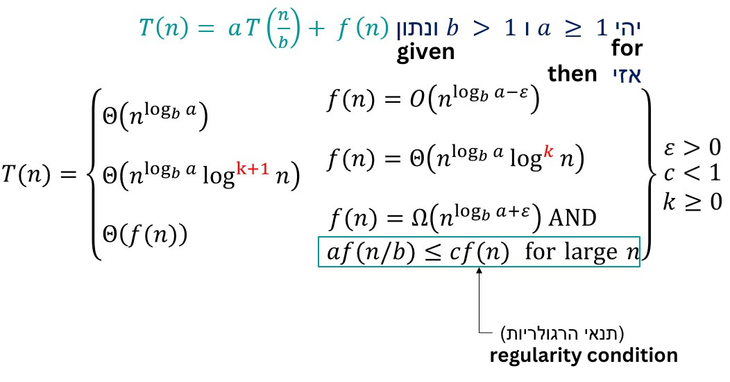
- Constants: a >= 1, b > 1
- F(n) > 0
- Check n^log(b,a) _ f(n)
- Case 3:
- af(n/b) <= cf(n) then t(n) = Θ(f(n))
- for c < 1
- regularity check
- af(n/b) <= cf(n) then t(n) = Θ(f(n))
Background for graphs
- Edge is a pair of 2 vertices
- G = (V,E)
- Graph G is defined as the ordered pair of a group of vertices V and edges E
- Directed graph
- Every edge is an ordered pair
- (v,u) != (u,v)
- we use arrows to differentiate and know the direction
- v -> u means a edge from v to u (but if we are in u, there is no way to get to v here, unless we add another edge)
- Undirected graph
- Every edge is an unordered pair
- {v,u} = {u,v}
|V|denotes the number of vertices in a graph|E|denotes the number of edges in a graph- d[u] denotes the detection/discovery time of vertex u
- f[u] denotes the finishing time of vertex u
-
π[v] denotes an array containing the predecessors of vertex v.
- Path = set of vertices (if undirected graph, the set will be unordered), where every edge between 2 vertices is a pair.
- Reachability = If there is a path from vertex U to vertex V (U⇝V), then V is reachable from U (in directed graph, U isn’t necessarily reachable from V)
- Simple Path = path where every vertex in path appears only once
- Cycle = path where V0 = Vn (first vertex is the same as the last vertex)
- smallest path that can make a cycle will have 3 vertices (if we don’t allow self loops)
- Simple Cycle = a cycle but the only repeated vertex is V0 = Vn
- Subgraph G’ = (V’,E’)
- where V’ ⊆ V, E’ ⊆ E
- All the vertices in the subgraph have to exist also in the original Graph (same as edges)
- Meaning we cannot add any vertex/edge to G’ that wasn’t already in G
- Spanning subgraph of G
- is a subgraph of G where V’ = V
- Graph G can be it’s own spanning subgraph
- may have fewer edges than G, but it has to cover all of the vertices of G
- Connected Vertices
- Two vertices are connected if there exists a path between them (undirected graph)
- Stringly Connected Vertices
- Two vertices are connected if there exists a path between them (directed graph)
- Connected Graph
- In an undirected graph where there exists a path between every 2 vertices (ie E - B)
- Strongly Connected Graph
- In a directed graph, exists a path between every 2 vertices (E <-> B)
- Sparse Graph = (
|E| = O(|V|))- Can remove edges, and as long as the number of edges is the same order of magnitude as the number of vertices… still will be sparse
- Dense Graph = (
|E| = Θ(|V|^2))- More vertices than edges (by an order of magnitude)
- Complete Graph =
- Edge between every 2 vertices (in undirected graph)
- Connected Component
- For undirected graphs
- Maximal, connected subgraph
- Maximal means no more vertices can be added to the subgraph to still be connected
- Strongly Connected Component (SCC)
- For directed graphs
- A strongly connected component is a maximal set of vertices C ⊆ V such that for every pair of vertices u and v in C, u and v are mutully reachable (both u⇝v and v⇝u)
- Tree
- Acyclic and connected graph
- Connected components of a forest = a tree
- Graph G = (V,E) is a tree iff G is acyclic and
|E|=|V| - 1 - Height of any complete tree is log(n) - base depends on # of children allowed
- Forest
- Acyclic graph
- a tree is a forest, but a forest isn’t always a tree
- its a graph and not a set of trees
- a subgraph of a forest = always a forest
Adjacency representation (for graphs)
| Representation | Find Edge (search) | Insert Edge (add) | Delete Edge (remove) | Memory (space) |
|---|---|---|---|---|
| List | O(|V|) |
O(1) |
O(|V|) |
Θ(|V|+|E|) |
| Matrix | O(1) |
O(1) |
O(1) |
Θ(|V|^2) |
-
List = for every vertex u in the graph, u has a list of vertices connected to it (node to neighbor)
-
In (binary) 2 dimensional matrix form, every row/column cooresponds to a vertex. The index will be 0 if there is not an edge between those two vertices.
-
If we are using a (linked) list, we insert an edge at the head of the list. Otherwise, we just go to the respective row and column in the matrix and flip the bit from 0 to 1
Vertex colors
- White: unprocessed/undiscovered
- Grey: processing/not finished
- Black: done/finished
Edge types
-
Let U be the parent, and V be the descendent
- Tree Edge
- Parent to a child
- Goes to undiscovered vertex
- V finishes before U
- U is grey, V is white
- Back Edge
- To an ancestor
- Of a vertex (parent, grandparent, etc.)
- Adding a back edge to tree edge makes a cycle
- To discovered but unfinished vertex
- In DFS, every back edge completes a cycle
- Removing back edges from a graph removes all cycles
- Self-edge = back edge
- V finishes after U
- To an ancestor
- Forward Edge
- To a non-child descendant
- To a finished vertex discovered after the current vertex
- Indirect descendant (not child)
- V finishes before U
- U is grey and V is black
- To a non-child descendant
- Cross Edge
- Everything else
- To a vertex finished before the current vertex’s discovery
- One branch to another tree, or one tree to another (ie 1 component to another)
- V finishes before U
- U is grey and V is black
- Everything else
White Path Lemma\Theorem
- ( V ) descends ( U ) iff at time ( d[u] ) there exists a path from ( u ) to ( v ) composed completely of white (undiscovered) vertices.
Parenthesis Theorem
- If ( V ) is a descendant of ( U ), then time ( d[v] ) is later than the time ( d[u] ). However, ( f[v] ) is earlier than ( f[u] )
| BFS (Breadth First Search) | DFS (Depth First Search) | |
|---|---|---|
| Approach | Explores level by level | Explores branch by branch |
| Data Structure | Uses a queue | Uses a stack or recursion |
| Memory Usage | Requires more memory | Requires less memory |
| Time Complexity | O(V+E) | Θ(V+E) |
| Use Cases | Shortest path in unweighted graph, reachable nodes from a starting node | Detecting cycles, exploring all nodes in a graph |
BFS
- Discover all vertices reachable from a starting source vertex
- Works for directed, undirected graphs
- Each iteration, go one level deeper in all possible directions
- Stop after reaching
- Queue = FIFO
DFS
- Dicover all vertices from a starting source vertex by going deeper in graph
- If we decide to go from left to right, go to S’s first neighbor from left… then go to it’s first left neighbor till you cant go further
- Then backtrack to the next possible path and continue
- Graph G is acyclic (has no cycles) if and only if the DFS produces no back edges
- if it’s directed, we call it a DAG (directed, acyclic graph)
- Undirected - complexity is O(V)
- Stack = LIFO
Topological Sort in DAG
- Order relation
- Puts all vertices in a sequence such that for every edge (U,V) in G, vertex U appears before V
- if graph has cycle (not a DAG) but also no linear/total order is possible
- Puts all vertices in a sequence such that for every edge (U,V) in G, vertex U appears before V
- Uses depth first search (DFS)
- DFS on G and get finishing times of all vertices
- as each vertex finishes, add to front of linked list
- return linked list of vertices
- Insertion is O(1),
|V|vertices to add - Usually we would want to reverse the linked list to get our prefered order
B tree:
-
2-3 Tree: Can have at most 2 keys, at most 3 children. They are a type of B tree
- Rules:
- All keys in node are sorted (i.e. left = smaller)
- Root node can have a minimum of 2 children (1 key is fine)
- Every node must fill at least half of their children ceil(m/2), node with degree 10 needs to have 5 children
- All leaf nodes must be at the same level (depth), thus tree is completely balanced
- no dangling nodes, leaves don’t have children
- Creation of nodes is bottom up (insertion) and grows upwards
- Stats:
- Depth of tree is order of log(n), operations (search, insert, etc.) are similar
- Number of keys in each node = from ceil(m/2) – 1 to m-1
- Number of children = number of keys + 1
- Minimal # of children = (ceil(m/2) – 1 (h+1)) / (ceil(m/2) -1)
- Maximal # of children = (m(h+1)) / (m-1)
- Number of leaves = from 2(ceil(m/2))^h to m^(h+1) -1
Easier way to understand:
- bounds from B to 2B-1
- B <= # of children < 2B
- B = branching factor (bound of number of children), for 2-3 tree B = 2
- either 2 children or 3 children
- non-leaf node with k children contains k-1 keys
- root has at least 2 children if not a leaf
- non-leaf node (besides root) has at least ceil(m/2) children
Hash Table & Functions:
- m = size of table
- h1(key) is the function that returns the index in the array for given item
- Table is indexed from 0 to m-1
- There are a lot of hashing functions, but the simplest used is usually h(key) = key % m
- the % m part assures that you cannot exceed the bounds of the table… given your key you will end up within the range of 0 to m-1
- Load factor of a hash table = total number of items stored in table / size of table = n/m = α
- Normally, each spot in the table can only hold a single element (and it’s key) - this is called direct addressing
- additionally, your key cannot end up in other slots
- With chaining specifically (part of open addressing):
- each spot has a linked list (empty by default), upon insertion, element becomes the new head of the list
- upon collision, the newer item gets put at the head of the list for the respestive spot and the previous item in the list becomes the node after the head.
- Open addressing allows your key to go to almost (if not all) of the slots by using a probe/step function
- i.e. for linear/quadratic probing we have a step function in addition to the original hash function, with a coefficient i/i^2 respective to the type of probe. Initially it will be 0, but after every collision we will increment by 1
- Linear probing:
- h(k,i) = (h1(k) + i) mod m
- f(i) = i
- Insert: first try, i = 0… if collision, set i = 1 and try to hash and insert again (can wrap around if necessary)
- Search: in for loop, i = 0 to m-1 hash the key with i then see if result in table = key
- if it does, return item. If entry is empty in table, return null… if slot was full but key didn’t match, then let i=i+1 and try again. If got to m-1 then return null as well
- Delete:
- run Search, if key found then mark as deleted, otherwise do nothing
- Mark as deleted but don’t delete as it would make it harder to find other elements that got same collision and were placed after it
- Quadratic probing:
- h(k,i) = (h1(k) + c1i + c2i2) mod m
- h1 is ordinary hash function, c1, c2 are constants
- Double hashing:
- given two hash functions, h1, h2, and i which starts at 0
- h = (h1(k) + ih2) mod m
- this is how you would usually map a item to a spot in the hash table
- if there is a collision, i gets incremented by 1 and compute the index via h again
- keep on doing this till you find an empty spot.
- if h2 is chosen/created in a poor manner (or h1, or table is small, or not sparse) etc… you can end up in an infinite loop looking for an open slot
More resources
Intro To Algorithms Solution Site - 3rd party